
I post-trained Qwen3-Coder-30B to fix bugs with an interactive debugger which lets the model set breakpoints and inspect runtime state. On the 30 test tasks, the final model (after RL) achieves 90.0% pass@3, up from 73.0% for the base model, and pass@1 rises from 55.8% to 72.9%.
I built a custom RL trainer in PyTorch for asynchronous rollouts and multi-GPU training, alongside the debugging harness, evaluations, and SFT data pipeline.
LoRA adapter · Inference Server / Harness
During my first co-op while at the University of Waterloo, my manager questioned why I was debugging with print statements and introduced me to an interactive debugger. Since then, I've preferred using a debugger over print-debugging, whether in IDEs or in the terminal.
Debuggers are uniquely useful because they can:
- See the call stack and variables across frames instead of relying on incomplete print logs.
- Evaluate expressions and alter execution live, without rerunning/recompiling or modifying source.
- Pause at an exception or step into third-party code with the current runtime context intact.
So what happens when I give a language model a debugger? That question forms the basis of this research project.
Baseline evaluations
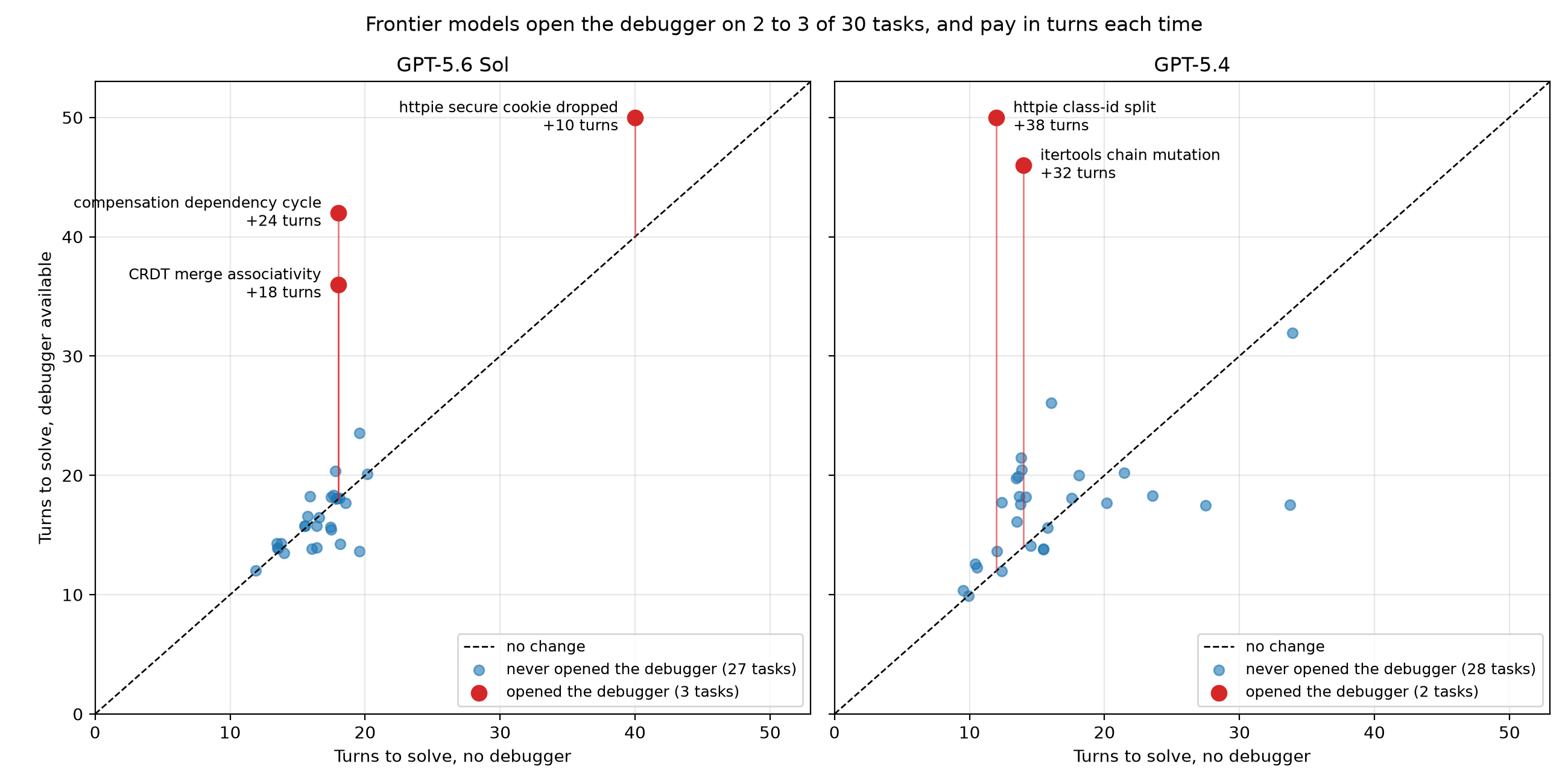
I ran baseline evaluations on GPT-5.4 (a frontier model at the time) and recently reran them on GPT-5.6 Sol. Neither model used the debugger effectively on these 30 tasks (Figure 1) – both spent extra turns on debugger use that was essentially unproductive.
GPT-5.6's introspection was redundant and sometimes incorrect (issuing pdb commands that raised errors), and episodes where it used the debugger took on average 17 extra turns compared to the ones that used only bash.
GPT-5.4 was worse; it took an additional 32 and 38 turns on the two tasks where it used the debugger, wasting turns on breakpoints set on non-executable/unreachable lines and inspecting variables before they were defined. In those episodes, the program finished without stopping at a breakpoint, and the model ultimately fixed the bug by falling back to bash.
Debugger use was also rare for both models and came late in the episodes: GPT-5.6 opened it on three of the 30 tasks, and GPT-5.4 on two. Those episodes used two to five times as many tokens as their bash-only counterparts, with the same outcomes.
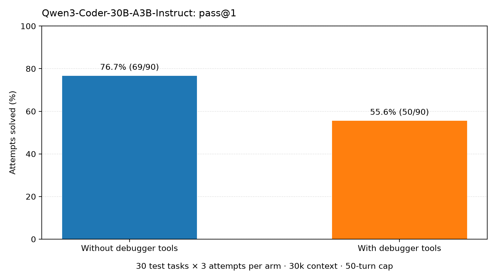
Evaluating Qwen3-Coder-30B-A3B-Instruct showed the opposite failure mode. It opened the debugger in 90.8% of episodes, but often continued investigating instead of making a fix. Comparing across the same 30 tasks, with three episodes each, giving it debugger access lowered the solve rate from 76.7% to 55.6% (Figure 2).
Throughout this post, “Base” refers to Qwen3-Coder-30B-A3B-Instruct before any of my SFT and RL training.
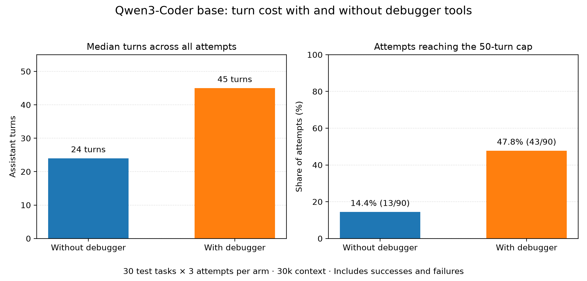
Qwen3-Coder-30B-A3B-Instruct also spent a greater number of turns per episode. Median turns rose from 24 to 45, and nearly half of debugger-enabled episodes reached the 50-turn cap (Figure 3). These counts include both successful and failed episodes.
Giving Qwen a debugger made it investigate more and solve fewer bugs. Could post-training teach it when to inspect runtime state, and how to turn that information into a fix? I used supervised fine-tuning to teach the workflow, then reinforcement learning to make successful episodes more frequent.
The trained debugger in action
Here is the final RL-trained policy on two held-out tasks.
In the following task, modifying a copy of a variable also modified the original. The trained model adds a breakpoint inside the correct file (with the bug), introspects execution efficiently, and fixes the bug correctly.
The trained model solves the bug much more efficiently at 24 assistant turns, while the base model hit the 50-turn budget.
On another task, the model reproduces the failure, introspects the suspected bug and then performs an edit that passes tests, finishing in 16 turns.
These trajectories showcase the behaviour I wanted to teach. Form a concrete hypothesis, inspect it, use what you find to make a fix, and then test the result.
What changed after training
After finishing SFT and RL post-training, the trained policy's pass@1 rose from 55.8% to 72.9%, and pass@3 rose from 73.0% to 90.0% (compared with the base model given the same tools).
For each evaluation, I sampled eight episodes per task (240 episodes total) in the same harness, with a 30k context and a 50-turn cap. An episode was successful if it passed the task's defined tests.
The comparison below follows the checkpoints used for the final RL run. Its SFT initialization scored 67.5% pass@1, and RL raised that to 72.9%, a gain of 5.4 percentage points.
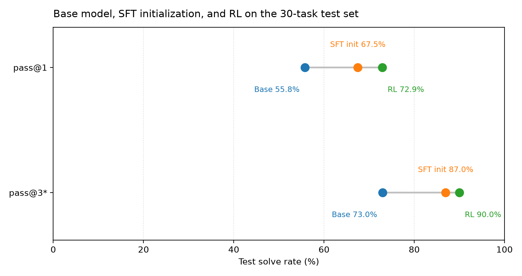
| Measure | Base | SFT initialization | Final RL |
|---|---|---|---|
| Single-episode solve rate (pass@1) | 55.8% | 67.5% | 72.9% |
| Solve within three episodes (estimated pass@3*) | 73.0% | 87.0% | 90.0% |
| Tasks solved at least once in eight episodes | 25/30 | 30/30 | 29/30 |
| Episodes that never edited a file | 37/240 | 10/240 | 0/240 |
Pass@3* is estimated over every three-episode subset of the eight. Compared with its SFT initialization, the final RL checkpoint solved fewer tasks at least once across eight episodes (29 versus 30), but had higher estimated pass@3.
The RL checkpoint was selected using a sweep on the test split, so these test results are not an independent estimate of generalization.
The harness and RL/eval environment
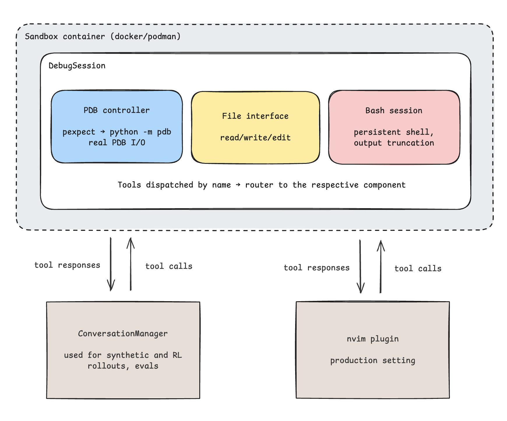
A robust harness was essential for baseline evaluation, collecting SFT demonstrations, and most importantly, RL rollouts. Each episode begins in a fresh sandbox with buggy Python source, supporting files, and visible tests.
Supported tools
The harness exposed tools to read and edit files, run shell commands and tests, and control a real pdb session exposed through structured tools. Unlike traditional (stateless) harness tools, breakpoints, stack frames, and execution context persisted across turns. Instead of simply passing through tool call results, the harness filtered and bounded tool call output so the model could condition its next action on the relevant runtime state, rather than noise like Python's internal module metadata (__name__, __loader__, __spec__) and large __builtins__ dumps.
Tasks that make runtime inspection useful
For both evaluation and training data, I constructed bug tasks that would benefit from a debugger – tasks involving shared state, serialization, concurrency, and other lifecycle bugs. For example, one task involves a re-entrant lock that hangs because it stores its owner as a thread object but compares it with an integer thread ID.
The files below show the lock implementation and the tests that expose the hang:
1import os
2import sys
3import threading
4import time
5
6sys.path.append(os.path.dirname(__file__))
7
8from resource import SharedResource
9from callback import CallbackChain, WorkItem
10
11
12class ReentrantLock:
13    def __init__(self):
14        self._lock = threading.Lock()
15        self._owner = None
16        self._count = 0
17        self._condition = threading.Condition(threading.Lock())
18
19    def acquire(self, timeout=None):
20        me = threading.current_thread().ident
21        deadline = None if timeout is None else time.monotonic() + timeout
22
23        with self._condition:
24            if self._owner == me:
25                self._count += 1
26                return True
27
28            while self._owner is not None:
29                if deadline is not None:
30                    remaining = deadline - time.monotonic()
31                    if remaining <= 0:
32                        return False
33                    self._condition.wait(timeout=remaining)
34                else:
35                    self._condition.wait()
36
37            self._owner = threading.current_thread()
38            self._count = 1
39            return True
40
41    def release(self):
42        with self._condition:
43            self._count -= 1
44            if self._count == 0:
45                self._owner = None
46                self._condition.notify()
47
48
49class ResourceGuard:
50    def __init__(self, resource=None):
51        self.resource = resource or SharedResource()
52        self._lock = ReentrantLock()
53
54    def read(self, key, timeout=None):
55        if not self._lock.acquire(timeout=timeout):
56            raise TimeoutError(f"Could not acquire lock for read({key})")
57        try:
58            return self.resource.read(key)
59        finally:
60            self._lock.release()
61
62    def write(self, key, value, timeout=None):
63        if not self._lock.acquire(timeout=timeout):
64            raise TimeoutError(f"Could not acquire lock for write({key})")
65        try:
66            self.resource.write(key, value)
67        finally:
68            self._lock.release()
69
70    def read_then_write(self, key, transform, timeout=None):
71        if not self._lock.acquire(timeout=timeout):
72            raise TimeoutError(f"Could not acquire lock for read_then_write({key})")
73        try:
74            current = self.read(key, timeout=timeout)
75            new_val = transform(current)
76            self.write(key, new_val, timeout=timeout)
77            return new_val
78        finally:
79            self._lock.release()
80
81
82class LockManager:
83    def __init__(self):
84        self._guards = {}
85
86    def get_guard(self, name):
87        if name not in self._guards:
88            self._guards[name] = ResourceGuard()
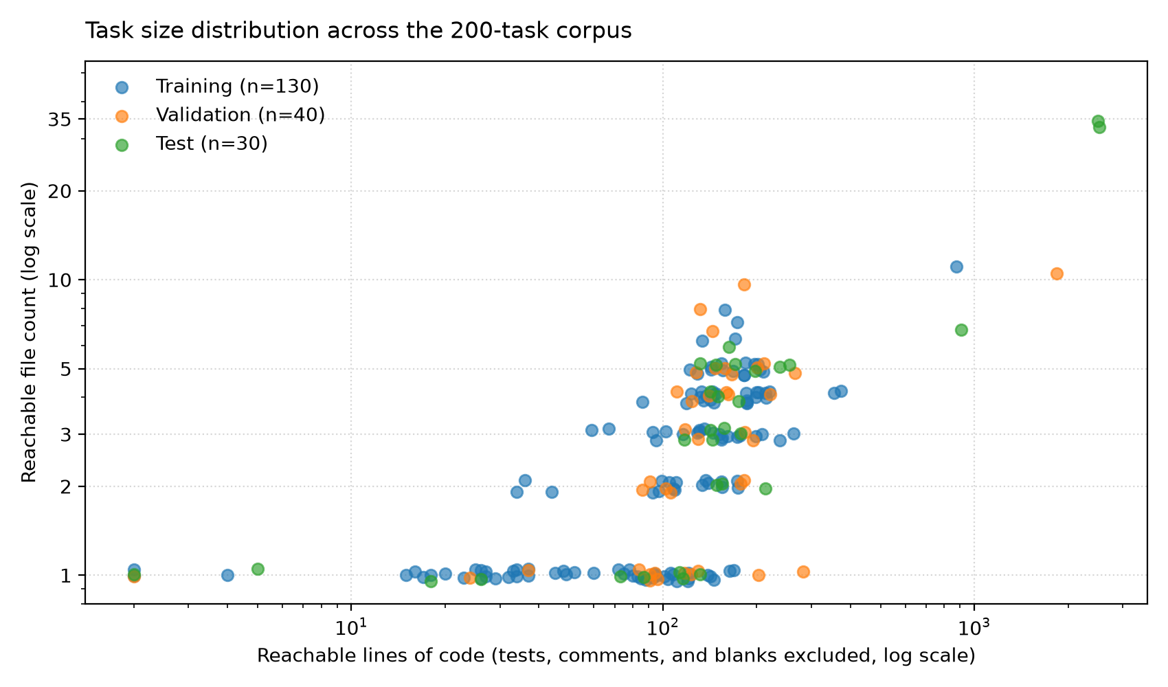
89 return self._guards[name]The median task contained 132 lines of Python source across three files reachable through direct or indirect imports from the failing test (Figure 6).
Building the supervised corpus
The first step in post-training my selected base model to use a debugger effectively was supervised fine-tuning on high-quality demonstrations.
Qwen3-Coder-30B-A3B-Instruct is a sparse MoE with 128 experts, 8 routed per token, and ~30B total parameters but only ~3B active on each forward pass. With only a few hundred trajectories in the final train split, I was concerned about catastrophic forgetting from full-parameter fine-tuning. Instead, I chose to use parameter-efficient training (LoRA1)2. Schulman et al.3 show that LoRA can match full fine-tuning in many post-training settings.
Generating and filtering trajectories
Because the task is multi-turn, each SFT example contains the complete debugging trajectory, represented as a sequence of tool calls interleaved with reasoning.
Here's an example trajectory:
1T1   bash:               ls                                # inventory the workspace
2T2   bash:               wc -l *.py                        # size files before reading
3T3   bash:               pytest -xvs test_file.py          # reproduce the failure
4T4   bash:               grep -n "def suspect" module.py   # locate code before reading
5T5   bash:               sed -n '40,90p' module.py         # read a bounded range
6T6   (reasoning)                                           # form a concrete hypothesis
7T7   start_debugger:     test_file.py, test_failing_case   # run only the failing test
8T8   add_breakpoint:     module.py:62                      # target the hypothesis
9T9   continue_execution                                    # advance to the breakpoint
10T10  examine_locals                                        # inspect runtime evidence
11T11  print_variable:     entry.calibration                 # read the one suspect value
12T12  step_over                                             # advance one statement
13T13  print_variable:     entry.calibration                 # see what that statement changed
14T14  step_into                                             # follow the call that mutates it
15T15  where_am_i                                            # confirm the frame after the jump
16T16  run_expression:     [c.calibration for c in pool]     # test the hypothesis directly
17...                                                        # keep stepping while each call
18                                                           #   changes the diagnosis
19T24  edit_file:          module.py                         # make a focused patch
20T25  bash:               pytest -xvs test_file.py          # verify before done
21...                                                        # still failing: form a new
22                                                           #   hypothesis and return to T8
23T38  done                                                  # only after a passing run
My initial data recipe utilized teacher-generated demonstrations, for which I used MiniMax M2.5 because it was affordable and performed well on coding tasks. I had also considered Kimi 2.6, but MiniMax M2.5 turned out to be a better teacher because it had better instruction-following and produced passing traces more reliably. I generated trajectories through the same DebugSession harness and kept only those that passed the tests and other criteria.
Microskills and training objective
While I had full demonstrations to use for fine-tuning, a useful action sequence might appear only once in each of these trajectories. To give the model more training signal for specific habits, I added supplementary short "microskill" SFT examples:
- read before editing
- debugger discipline (breakpoint placement, introspection, etc.)
- rerun
pytestbeforedone - recover from a failed edit
The first training corpus had 527 entries: 279 full fix trajectories and 248 microskills. Later runs replaced it with the final corpus described in the next section, which kept only verified fixes and included more examples of the task types the model kept failing.
For SFT, I masked user and tool messages out of the training loss, so I computed the loss only on assistant tokens. Thus, the model learned from every assistant action I kept. Trajectories were filtered by more than just their passing tests; I also filtered for the behaviours described below.
What actually improved the checkpoint
The fixed train/validation/test split assigned 130 tasks to training, 40 to validation and recipe iteration, and 30 to the test split for selected policies.
Between SFT runs, I repeated this loop:
- Train a checkpoint.
- Evaluate it on the validation-split tasks.
- Inspect the trajectories for any failure modes.
- Change the corpus or the data preprocessing to correct them.
When an SFT checkpoint showed promising performance after step 3, I used it for a subsequent RL training run. If RL exposed failure modes that were better addressed in the SFT phase, I repeated the loop and updated the SFT checkpoint before restarting RL from the new (and improved) SFT init.
Adding demonstrations of successful solutions expanded what the model could do. Filtering mostly prevented it from learning bad habits. Below are four components of the SFT recipe I investigated and their effects on validation performance.
1. Preserve both efficient solutions and recovery behaviour
For SFT, I had both long successful trajectories and short successful trajectories to choose from. While short trajectories taught efficient debugging, the longer ones taught recovery and repeated attempts before reaching a correct fix. I found that mixing short and long examples was beneficial: the model could learn efficient fixes while still seeing how successful debugging sessions continued over many tool calls. To do this, I alternated between the shortest and longest successful trajectories, working inward:
1group.sort(key=lambda row: row.turns)
2
3while lo <= hi:
4    picks.append(group[lo])       # efficiency exemplar
5    if hi != lo:
6        picks.append(group[hi])   # long-horizon coverage
7    lo, hi = lo + 1, hi - 1
To showcase the difference between trajectories and the value in each:
The long route is not an efficiency exemplar. It preserves recovery behavior: observe a failed patch, back out, gather new evidence, and still finish verified.
Figure 7: Two selected fixes for the same training task. The longer route is not presented as ideal, but it retains a kind of recovery behaviour absent from the seven-call solution.
With this change, the model reached 59.1% pass@1 and 79.5% pass@3* over eight episodes, up from 53.3% and 70.0% in run 2 (+5.8 and +9.5 points), which was the strongest checkpoint produced up to that point.
2. Process matters just as much as the outcome
It’s important to look at the trajectories you’re using for SFT, since every assistant token in a trajectory gets equal supervision. A trajectory can reach the successful outcome (passing tests) while taking “bad” actions along the way. If you only filter on the outcome, that bad behaviour makes its way into the trained policy. In fact, outcome-filtered SFT doesn’t just tolerate bad intermediate behaviour. It can selectively amplify the bad behaviour that helped the trajectory pass.
To filter trajectories, I rejected invalid tool ordering, blind stepping, repeated loops, edits without a prior read, debugger observations that did not inform the edit, and a done tool call before verification.
In simplified form:
1if debugger_share > max_debugger_share:
2    reject("debugger treadmill")
3if debugger_streak > max_debugger_run:
4    reject("consecutive debugger run")
5if first_source_edit > 0.75:
6    reject("late source edit")
7if require_final_verify and not final_verified:
8    reject("final source edit was never retested")
Surprisingly, this change did not result in better downstream evaluation performance. I expected it to, since cleaner trajectories without incorrect/wasteful actions should intuitively give the model a more direct path to the outcome. My best guess is that filtering can remove bad habits, but it can’t add solutions the teacher never found.
I kept the filters as quality checks even though they didn’t move pass@k.
3. Harvest complementary discoveries from changing policies
When the later SFT checkpoints had learned a better debugger-use policy, I used an on-policy STaR loop4.
To do this, I ran the current best policy on the training split and added its successful trajectories to the supervised corpus. Unlike standard STaR with an answer key, the independent verifier here executes the repository's tests and the behavioural gates (from the previous section) reject valid-but-undisciplined traces.
In later runs, the strongest policy was an RL-trained checkpoint that solved new tasks the base and SFT models could not. Its successful trajectories were then added as demonstrations for the next SFT checkpoint.My final SFT data mix drew from three policy generations. The base model contributed different ways to solve the tasks, SFT checkpoints contributed examples of the intended debugging workflow, and RL-trained policies supplied fixes for harder task classes that earlier policies had not solved.
Figure 8: Contributions to the 312 training examples: 49 from Base, 127 from SFT models, and 136 from RL models. Slice labels count demonstrations, not distinct tasks.
4. Add tasks that target incorrect fixes
Before the final SFT round, I evaluated the strongest RL checkpoint to identify the remaining failure modes.
In that evaluation, 50 of 88 validation-task failures were caused by the model arriving at an incorrect fix. To address this, I added six training-split tasks where the most obvious fix could still leave other tests failing, to teach the model to address the full bug rather than just its immediate symptom.
As a result of these added tasks, the best RL-trained checkpoint contributed 19 examples across these tasks for the next SFT corpus.
The final corpus
The final SFT corpus contained 347 trajectories spanning 116 of 130 training tasks. Of these, 312 were used for training and 35 were held out.
Comparing Base vs SFT on the same task
This test-split task models a lease gateway for incoming requests. The bug in the task is that a request that failed validation still acquired a lease, and its handler returned early and didn't register it.
Below, the comparison shows how Base and SFT handled this bug. Both set breakpoints on the request path, but only SFT placed one where it could compare a valid request with a rejected one.
In both trajectories, the model reproduces the failure at turn 2 (running tests) and starts the debugger at turn 7. What differs is their efficiency thereafter.
Base breaks at the top of the request loop and steps through every line of the first request. It reaches the size check for the rejected request at turn 50 and never edits the code. Base did not solve this task in any of its eight episodes, and five of those episodes ended without an edit.
On the other hand, SFT cleverly breaks inside Worker.serve, allowing the model to introspect for each request. At the second stop, it sees the size-0 request raise AdmissionError and return before outcome.finish(...). It applies the fix at turn 21, reruns the failing test and then all seven tests, and submits the fix at turn 24. The SFT checkpoint solved this task in two of eight episodes.
With this more reliable bug-fixing policy, RL was more likely to generate successful trajectories it could learn from.
What did not matter as much as I expected
Passing the failing test name into the debugger. In run 5, I let the model start the debugger on a specific test which raised targeted starts from 63% to 99%. But pass@1 did not meaningfully improve; run 5 was 54.4%, compared with 55.6% for run 4. Debugger sessions also grew from 14.3 to 16.6 calls on average, but this isn't necessarily a negative signal.
Stricter trajectory filtering. Removing debugger treadmills, late edits, and unverified fixes did not produce a retrain that beat prior runs. Filtering removed bad examples without adding better ones to learn from.
SFT results
Validation: reliability and observed coverage
For evaluation, I ran eight episodes per task with a 30k context and a 50-turn budget, using those episodes to estimate pass@1 and pass@3. These scores don't directly show coverage: how many tasks the model solved at least once across all eight episodes. Figure 9 shows how that coverage changed across the SFT checkpoints I used to develop the corpus.
Figure 9: Base and three SFT checkpoints from corpus development across eight episodes on 40 validation tasks. Tasks solved at least once grew from 36 to 39; tasks solved in every episode grew from 5 to 12.
The last of these checkpoints reached 67.2% pass@1 and 88.6% pass@3*, versus 48.8% and 72.8% for base. It solved 39/40 tasks at least once and 12/40 in every episode, compared with 36 and 5 for base; never-edit failures fell from 82/320 to 24/320.
Compared with the earlier SFT checkpoint, the final checkpoint failed less often by repeating debugger calls. Wrong fixes accounted for more of its remaining failures.
Test: comparison with Base
The SFT checkpoint used to initialize the final RL run reached 67.5% pass@1 and 87.0% pass@3* on the 30-task test set, across eight episodes per task, against 55.8% and 73.0% for the base model. It solved 30/30 tasks at least once, versus 25/30 for the base model.
The validation and test sets were balanced by difficulty and debugger preference, but contained different tasks.
Using RL to improve reliability
I used SFT to give the model a strong enough starting point to follow complete debugging workflows before beginning RL. I then used a modified version of Group Relative Policy Optimization (GRPO)5 to let it learn from experience instead of just imitation. This division of roles echoes Chu et al. (2025), who found that SFT established reliable output structure while RL improved generalization on their reasoning tasks.
What changed between SFT and RL on the same bug
The next comparison shows trajectories from the final SFT checkpoint and the final RL checkpoint. The task is deepcopy_circular, which has a bug where changing a copied scene's nested payload also changed the original. The RL trajectory here is a different episode from the 24-turn video above; this one finished in 27 assistant turns. Both policies inspected the same part of the copy routine at turn 11 but made different fixes. SFT reused a cached payload that still pointed to the original; RL changed how the cache was populated so it held a deep copy.
Both episodes used a 30k context, a 50-turn limit, and temperature 0.1.
The GRPO recipe
RL started from the SFT initialization in Figure 4, which scored 67.5% test pass@1.
The run also used an adaptive KL penalty against a reference policy and a behaviour-cloning anchor with replay seeded from the SFT corpus, to help retain the workflows learned during SFT.
Instead of using the version of GRPO as it was presented in the DeepSeekMath paper, I made three changes to the update: removed reward-standard-deviation scaling, used asymmetric clipping, and added mild trajectory-length weighting. I discuss the rationale in more detail below.
Group and batch size
Across 130 training tasks, the final run targeted four groups of 12 trajectories per optimizer step, with all trajectories in a group coming from the same task/prompt. A full update therefore used 48 trajectories while combining learning signals from multiple tasks.
The run's hardware profile fixed the dynamic group-size range at 12, overriding the general configuration's maximum of 16. Timeout handling could also seal partial groups with at least eight trajectories, so some updates used fewer than 48.
Choosing training tasks
As mentioned above, avoiding low-variance groups leads to fewer wasted rollouts during RL. Said another way, training favors tasks the model can solve sometimes, but not consistently. These tasks are more likely to produce both successful and failed attempts within a group, giving GRPO a useful comparison for learning which actions lead to a correct fix. In my recipe, tasks with estimated success rates of 30–70% accounted for 46% of training rollouts.
The curriculum had two discrete phases with variable difficulty within each: debugger acquisition, followed by debugger abstention.
I started with 80% debugger-recommended and 20% optional tasks, then introduced avoid tasks to teach when to skip the debugger. Advancement depended on successful fixes and appropriate debugger use, including abstention, rather than mean reward alone. Difficulty increased within each category, and repeatedly unsolved tasks were sampled less often, with occasional retries as the model improved.
Policy updates
In this setup, an all-fail GRPO group can have a low reward standard deviation, so dividing by it can amplify small differences in process rewards during the training update. Following Dr. GRPO6, I removed this division to keep those differences small relative to the reward gap for a verified fix.
The change from standard GRPO is:
Here, is the trajectory's total reward; and are the group's reward mean and standard deviation, and the small constant prevents division by zero.
For a simplified example, compare two groups of two trajectories. In the first, both fail, but one earns slightly more process credit. In the second, one fails and one fixes the bug:
| Group | Rewards | With std division | Without std division |
|---|---|---|---|
| Two failures | 0.10, 0.12 | ≈ −1, +1 | −0.01, +0.01 |
| Failure and verified fix | 0, 1 | ≈ −1, +1 | −0.5, +0.5 |
In this simplified example, dividing by each group's standard deviation makes tiny process bonuses between failures as influential as fixing the bug. Removing that division keeps the learning signal proportional to the reward improvement.
Another change I made was to use asymmetric clipping, following DAPO7. Without it, the symmetric clip cut off learning signals from rare high-reward trajectories even while policy drift (KL) stayed below its threshold. I widened only the upper threshold, allowing more reinforcement of better-than-average trajectories:
Here, is the probability ratio between the current and rollout policies. Clipping limits the learning incentive, not the actual probability change.
The third change was mild trajectory-length weighting. For each trajectory, I counted its generated response tokens across all turns, then multiplied its advantages by:
Here, is the trajectory's generated-token count, with a minimum of one, and is the mean across the group. The weights have mean one: shorter trajectories receive somewhat more weight, and longer ones somewhat less. This changes the magnitude of both positive and negative advantages; it does not add a reward for being short. The loss averaged tokens within each response, then averaged response losses across the group. This length weighting is separate from the off-policy correction below.
I used asynchronous RL, which meant that a response could have been generated by an older policy by the time it reached the learner. To account for this, I stored each response’s token log probabilities and policy version, then computed each token’s importance ratio as the current policy’s probability divided by its stored rollout probability. This tied the PPO update to the policy that actually generated the response.
I also weighted each response by , where the mean is over that response's generated tokens. This length normalization makes equal average token-level drift receive the same weight regardless of response length. The configured clipping and maximum-ratio limit together bounded the weight to 0.1–5.0. This adjustment was separate from both PPO clipping and the trajectory-length weighting above. To limit policy drift, I excluded steps more than four policy versions old and rejected stale groups before training, though I did not ablate this.
In another earlier run, a process guard that stopped a degenerate episode also spared it the failing-test, turn-cap, and most turn-cost penalties. So the policy learned that the cheapest way to fail was to stall until a guard stopped the episode. Below, I compare two trajectories from failed episodes on the same task, in the same GRPO group, that showcase this behaviour.
Trajectory A did less useful work, but it scored 2.5 points higher, and GRPO reinforced it over B:
Trajectory A still earned credit for an inspection followed by an edit (+0.20), for its debugger choice (+0.15), for localization (+0.10), and for code changes (+0.05), although neither edit changed anything. Trajectory B made real edits and ran the tests, and lost 1.00 for failing tests and 0.50 for the turn cap. Inside the group, the update pushed the policy toward A. Across that run, failed episodes that a guard stopped averaged +0.095, against −0.949 for failed episodes that reached the turn cap on the same tasks.
These reward hacks showed that tool use and cheap failures could earn rewards without progress toward a fix. The final recipe limited process credit on failures, protected successful completions with a reward floor, and explicitly penalized guard exits.
The main bounds and termination penalties were:
| Rule | Value |
|---|---|
| Test-outcome reward weight | 1.00 |
Minimum total reward after passing tests and an accepted done | +0.45, applied after penalties |
| Positive process-credit cap on an unsolved episode | +0.35 |
| Higher process-credit cap on an unsolved episode after an informed edit followed by a test | +0.60 |
| Unfixed episode with no test progress | −0.50 terminal component |
| Failed episode that reached the turn cap | −0.50 component |
| Failed episode stopped by a stall guard | −0.65 component |
The last two penalties could be reduced by up to 50% for measured test progress. A separate turn-cost term had weight −0.20 and a capped cost of 1.4, for a maximum deduction of 0.28. These values are components and bounds, not complete episode rewards: test outcomes, repair progress, and other process terms also contributed. In particular, the process-credit caps did not guarantee that every failure scored below every success.
RL training setup
My RL system consisted of a learner, an inference server, a coordinator, and many asynchronous CPU workers running the debugging harness.
The diagram shows the 3-GPU setup:
Asynchronous GRPO
3 H200s · 32 sandbox environmentsI used FSDP to shard the Qwen3-Coder-30B-A3B-Instruct model across two H200 GPUs, with LoRA adapters on each. After each update, the learner sent the new adapter to the inference server via NCCL.
The inference server ran on the third H200. It used vLLM to generate the next model response for each CPU worker. Each worker maintained an episode in an isolated sandbox, executing tool calls to debug, edit files, and run tests.
A coordinator organized the training work between the FSDP learner and the CPU workers. It assigned tasks to workers, grouped completed trajectories from the same task, and forwarded those groups to the learner for training.
Why use FSDP?
Initially, my learner ran on a single GPU, which limited training to 6,144 tokens due to memory constraints. I checked the validation trajectories of the post-trained model and found that only 71.2% of successful trajectories and none of the failures fit within that limit. To train on longer debugging trajectories, I needed more memory.
Adding a second learner GPU increased total memory, but ordinary data parallelism would still keep a full copy of the model on each GPU. It would distribute training examples without freeing the memory needed for a longer sequence. Even with LoRA, the frozen 30B-parameter base model occupied most of the learner's memory, so splitting those weights was the main opportunity to make room.
To that end, I used Fully Sharded Data Parallel (FSDP) to shard the base weights across the two learner GPUs while letting both GPUs process different training inputs. Each GPU keeps one shard of each managed layer's weights, gathers the complete weights when it needs to compute that layer, and releases the gathered copy afterward. This saves memory between layer computations while distributing the training work across both GPUs, at the cost of communication to gather the weights.
With the base weights sharded, I could raise the training context to 16,384 tokens. That covered 96.3% of successful trajectories and 49.4% of failures in the audit, so fewer long debugging attempts were excluded from training. Sharding the base weights across more GPUs could have freed additional memory for longer training sequences.
What each GPU stores
Figure 12 paints a better picture of how FSDP lays out the base model and LoRA adapters across the 2 GPUs.
In my setup, FSDP sharded only the frozen base weights, and each GPU kept a copy of the LoRA adapter. Before gradient clipping, the two GPUs averaged the adapter gradients with one all-reduce. The reference adapter shared the policy’s frozen base weights, so reference scoring did not require a second copy of the base model.
Before
6,144-token training context
After
16,384-token training context
I chose to keep a full copy of the LoRA adapter on each GPU to avoid a problem with how FSDP handles frozen and trainable weights occupying the same layer. The usual setup wraps each decoder layer in one FSDP unit, which flattens its parameters into a single tensor. That did not fit my setup. Even though only the adapters need the gradients, FSDP keeps and reduces gradients for the full tensor. When profiling one update, I saw that each GPU reduce-scattered 30.1 billion elements across one forward and backward pass, despite only 104 million parameters being trainable.
Another approach would have been to wrap each LoRA module in its own FSDP unit to separate the trainable parameters from the frozen weights. This would have created thousands of small FSDP units, each requiring its own communication between GPUs. The full set of adapters occupies only 0.19 GiB in BF16, so keeping a copy on each GPU was simpler.
Why FSDP1, not FSDP2
I used FSDP1 because the expert kernels, vLLM weight transfers, and PPO scorer access weights directly. FSDP2’s distributed tensors caused failures and slower fallbacks in these paths. FSDP1 with use_orig_params=True kept the plain tensor views and parameter names my code expected.
Dealing with the expert layers
The standard Qwen3-MoE layer runs its 128 experts with a Python loop. Using the same grouped GEMM idea, I replaced the loop with grouped matrix multiplications: each layer sorts tokens by expert, then runs all experts in one kernel per projection.
This also required changing how I stored the LoRA weights. PEFT keeps each expert's A and B matrices in separate tensors, while the grouped kernels need them packed together. I packed the matrices across experts into one tensor for each layer, projection, and matrix type (A or B).
The grouped kernels also need a token count for each expert. In PyTorch 2.11, torch.bincount copies the input’s minimum and maximum to the CPU, forcing it to wait for queued GPU work in every layer. Since the router always chooses from 128 experts, I used a fixed-size scatter_add_ to compute the counts, avoiding that host-device synchronization.
Splitting work across the two GPUs
To keep the GPUs fed efficiently, I grouped steps that extended the same token sequence into chains and packed them into microbatches of at most 16,384 tokens. I then assigned the largest microbatches first to the GPU with the least work, balancing both token counts and the number of microbatches assigned to each GPU. Each GPU received roughly the same number of microbatches, with at most one extra on either side, to minimize rounds where one GPU only participated in synchronization while the other did useful work. This mattered because the GPUs synchronized between microbatch slots: the slower GPU determined how soon both could start the next slot.
Learner performance
Together, these changes made the learner 3.03x faster on a fixed workload of eight GRPO groups at 16k context, using the same inputs and starting weights. Peak GPU memory increased from 115.0 to 120.6 GiB.
Training throughput and serving
For this project, I used asynchronous RL, following the approach in PipelineRL8. Rollout workers collected debugging trajectories through a shared inference server, and the learner trained on completed GRPO groups when there was sufficient data. Keeping this pipeline supplied required balancing rollout generation, inference, and training.
As the learner advanced, rollouts could come from older policies. The importance weighting described in the GRPO recipe accounted for this mismatch, while a policy-lag limit excluded stale data.
Episodes varied in length, so I used a continuous pool of environments: when one episode finished, its slot immediately started another instead of waiting for the rest of a batch. While one environment executed tests or debugger commands, others could request their next model response.
In the vLLM inference server, I used continuous batching so that requests from different episodes could be processed together as they arrived. I also used prefix caching to reuse computation over repeated conversation history.
To feed the learner promptly, I had the coordinator prioritize tasks closest to filling a GRPO group, accounting for episodes already in flight. This turned completed trajectories into groups the learner could consume sooner, instead of spreading work across many unfinished groups.
To keep rollout production from getting too far ahead of learning, the coordinator paused new episode assignments when the training queue reached its high-water mark. Episodes already running could finish, and new assignments resumed once the queue fell below a lower threshold. This kept the learner supplied without building a long queue of trajectories generated by increasingly old policies.
What the model learned, and what remains unsolved
On the test split, the final RL-trained model’s inspection-to-edit conversion rose from 73.6% to 98.4%, and median turns fell from 45 to 30.5. It had no never-edit failures. However, of the final model's 65 failed trajectories, 57 were wrong fixes that exhausted the turn budget.
done while failing, and 61 remaining failed repairs that exhausted the turn budget. Categories are assigned in that order.Five tasks accounted for 32 of those failures. On producer_consumer_shutdown, all eight episodes failed, seven with test timeouts. The policy kept patching, waiting for the timeout, and reverting. On toctou_file_check, the model edited the localized code in five episodes but still failed assertions.
While I improved the model’s performance with debugging tools, the base model without debugger tools still scored numerically higher, at 76.7% over 90 episodes versus final RL's 72.9% over 240.
Reflections
This was a very fun project because I got to improve a model in a dimension I set out to improve: using a debugger to understand a bug before trying to fix it. There is still plenty of room for improvement, but it was satisfying to read the rollouts and see successive policy versions pick up skillful debugger behaviour.
It also gave me an appreciation for the range of systems and infrastructure problems in the RL stack—from the harness to the RL trainer itself. Applying asynchronous RL, serving changing policies, fitting long trajectories into GPU memory, and making distributed training efficient were all valuable learnings and important pieces of the project.
References
Edward J. Hu, Yelong Shen, Phillip Wallis, et al. "LoRA: Low-Rank Adaptation of Large Language Models." arXiv:2106.09685, 2021.
Neil Houlsby, Andrei Giurgiu, Stanislaw Jastrzebski, et al. "Parameter-Efficient Transfer Learning for NLP." arXiv:1902.00751, 2019.
John Schulman, in collaboration with others at Thinking Machines. "LoRA Without Regret." Thinking Machines Lab, 2025.
Eric Zelikman, Yuhuai Wu, Jesse Mu, and Noah D. Goodman. "STaR: Bootstrapping Reasoning With Reasoning." arXiv:2203.14465, 2022.
Zhihong Shao, Peiyi Wang, Qihao Zhu, et al. "DeepSeekMath: Pushing the Limits of Mathematical Reasoning in Open Language Models." arXiv:2402.03300, 2024.
Zichen Liu, Changyu Chen, Wenjun Li, et al. "Understanding R1-Zero-Like Training: A Critical Perspective." arXiv:2503.20783, 2025.
Qiying Yu, Zheng Zhang, Ruofei Zhu, et al. "DAPO: An Open-Source LLM Reinforcement Learning System at Scale." arXiv:2503.14476, 2025.
Alexandre Piché, Ehsan Kamalloo, Rafael Pardinas, Xiaoyin Chen, and Dzmitry Bahdanau. "PipelineRL: Faster On-policy Reinforcement Learning for Long Sequence Generation." arXiv:2509.19128, 2025.